Comparison of Clustering Performance for both CPU and GPU
Comparison of Clustering Performance for both CPU and GPU

A Benchmark: K-Means Algorithms for Scikit-Learn and TensorFlow-GPU
When you would like to have a deeper understanding of a phenomenon, one approach can be putting them in groups to make it easier to comprehend. As an example, you might want to view movies by title, while another person might view it by genre. How you decide to group them guides you to learn more about them.
In machine learning, dividing the data points into a certain number of groups is called clustering. These data points do not have initial labels. For that reason, clustering is the grouping of unlabeled data points into groups to figure them out in a more meaningful way.
There exist three kinds of clustering as Hierarchical Clustering (Divisive, Agglomerative), Partitional Clustering (Centroid, Model-Based, Graph-Theoretic, Spectral) and Bayesian Clustering (Decision Based, Nonparametric). In this post, we will be using Partitional Clustering>Centroid as the clustering algorithm.
For more deeper look for clustering techniques, please visit MIT-edu notes.
Throughout this post, the aim is to compare the clustering performances of Scikit-Learn (random, k-means++) and TensorFlow-GPU (k-means++, Tunnel k-means) algorithms by means of their execution times and print them in a comparison matrix by providing corresponding system specs. Since the content of the data is not the focus of this benchmark study, the required data sets will be randomly generated.
K-means Clustering
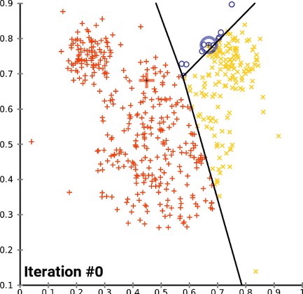
The purpose of k-means clustering is to partition some number of observations n into k number of centroids in a non-overlapping manner. The number of data points are expected to be as homogeneous as possible inside the cluster and as heterogeneous as possible outside the cluster. For more theoretical explanations, please kindly visit this webpage.
The algorithm works when a group of center points is available by following the below steps:
- Existing clusters are updated in order to include the nearest data points in distance to every centroid.
- The center points are iteratively recomputed as the average of all data points involving in a cluster.
Throughout this post, three different environments (2 different CPU-powered system, 1 GPU-powered system) will be tested. The system specs are added below.
First CPU-Powered System Specs:
Processor: Intel(R) Core(TM) i7–8850H
Processor Speed: 2.60 GHz
Physical Cores: 6
Logical Processors: 12
Physical Memory (RAM): 64 GB
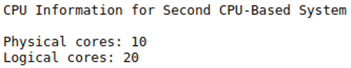
Second CPU-Powered System Specs:
Processor: Intel(R) Core(TM) i9–10900
Processor Speed: 3.70 GHz
Physical Cores: 10
Logical Processors: 20
Physical Memory (RAM): 256 GB (8 x 32GB DDR4 3000 MHz)
GPU-Powered System Specs:
Processor:Intel(R) Core(TM) i9–10900
Processor Speed: 3.70 GHz
Graphics Processors (GPU): NVIDIA GeForce® RTX 2080Ti 352-bit 11GB GDDR6 Memory (2)
1. CPU-based K-means Clustering
Central Processing Unit (CPU) is the crucial part computer where most of the processing and computing performs inside.
For the further coding part, we will be using the Python programming language (version 3.7). Both PyCharm and Jupyter Notebook can be used to run Python scripts. For the ease of use, Anaconda can be installed since it includes all required IDE’s and vital packages with itself.
As an initial step, we will be installing the required packages that will be required CPU implementation.
pip install psutil
pip install numpy
pip install matplotlib
pip install scikit-learn
After installing psutil, numpy, matplotlib, sklearn we will import the packages in order to be able to benefit from their features.
import platform
import time
import psutil as ps
import platform
from datetime import datetime
import numpy as np
import matplotlib.pyplot as plt
from sklearn.cluster import KMeans
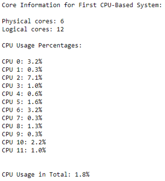
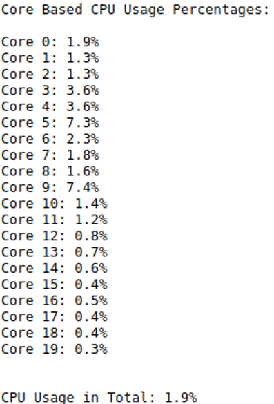
Before start clustering, CPU information and their current CPU usage percentages can be checked with the following code snippet.
print("Physical cores:", ps.cpu_count(logical=False))
print("Logical cores:", ps.cpu_count(logical=True),"\n")

print("CPU Usage Percentages:", "\n")
for i, percentage in enumerate(ps.cpu_percent(percpu=True)):
    print(f"CPU {i}: {percentage}%")

print("\n")
print(f"Current CPU Usage in Total: {ps.cpu_percent()}%")
There are two types of k-means algorithm that is existent within Kmeans() function with the parameter “init= random” or “init=kmeans++”. In below, firstly “init = random” which stands for selecting k observations in a random manner will be tested.
“n_clusters” parameter stands for the number of clusters the algorithm will split into. When we assign “n_clusters” into “100”, it signals algorithm to distribute all data points into most appropriate 100 centroids. To be able to control the randomness in every run, “random_state” parameter shall be set to an integer number; otherwise, a different random group will be selected in every run which will be harder to compare with the previous outputs.
kmeansRnd = KMeans(n_clusters=100, init='random',random_state=12345)
After setting cluster parameters, random numbers are generated with 5 columns and 500 K rows.
CPU_Test_1 = np.random.normal(size=(500000,5))
Now, we have 5-columned and 500 K-rowed randomly generated data. With “fit_predict” function, cluster centers and cluster indexes will be calculated for each data point by feeding our data named “CPU_Test_1”.
kmeansRnd.fit_predict(CPU_Test_1)
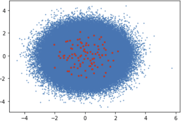
Visualization of the samples and the number of clusters are added by using “plotly” package of python. The results of this plotting script are added at the end of the system-based results in the upcoming sections of the post while depicting the data points and the clusters.
plt.scatter(CPU_Test_1[:,0], CPU_Test_1[:,1], s=1)
plt.scatter(kmeans.cluster_centers_[:,0], kmeans.cluster_centers_[:,1], s=5, c="r")
plt.title("K-means (Random) with Scikit Learn", "\n")
plt.show()
Execution times of the algorithms can be tracked by adding the following code lines outside of our algorithm.
start_time = time.time()
# ... clustering code block
end_time = time.time()
print(end_time - start_time)
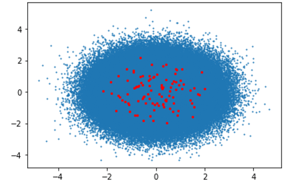
1.1. K-means (random) Clustering with Scikit-Learn
Scikit Learn K-means — random algorithm chooses the first center cluster in a random way which might cause a higher in-cluster variance compared to k-means++ algorithm.
First CPU-Powered System Results:
Algorithm Execution Time: 2505.26 seconds
Clusters Visualization: Blue Dots (Data Points), Red Dots (Clusters)
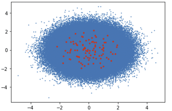
Second CPU-Powered System Results:
Algorithm Execution Time: 1395.10 seconds
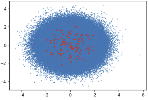
Clusters Visualization: Blue Dots (Data Points), Red Dots (Clusters)
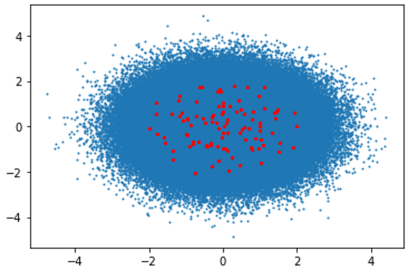
1.2. K-means (kmeans++) Clustering with Scikit-Learn
Scikit Learn K-means — kmeans++ algorithm chooses the first center cluster in a more logical way which can lead to a more accelerated clustering performance afterward.
First CPU-Powered System Results:
Algorithm Execution Time: 2603.74 seconds
Clusters Visualization: Blue Dots (Data Points), Red Dots (Clusters)
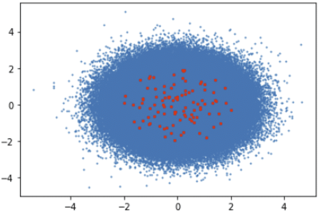
Second CPU-Powered System Results:
Algorithm Execution Time: 1384.73 seconds
Clusters Visualization: Blue Dots (Data Points), Red Dots (Clusters)
2. GPU-based Clustering
Tensorflow library is developed to be used for massive volumes of numerical computations. It supports both CPU and GPU according to the installed version of your environment. If you wish to enable your GPU(s), the version that is needed to be installed is TensorFlow-GPU.
pip install tensorflow-gpu
In order to be able to test the availability of GPU information by using TensorFlow library, the following code snippet can be used.
import tensorflow as tf
config = tf.compat.v1.ConfigProto()
tf.config.list_physical_devices('GPU')
Output:

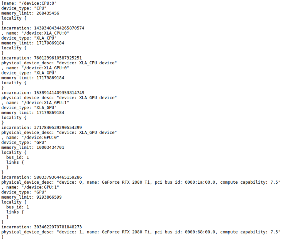
After viewing GPU information by using the below script, more detailed device information, including CPU(s), can be printed.
from tensorflow.python.client import device_lib as dev_lib
print (dev_lib.list_local_devices())
Output:
2.1. KMeansTF (kmeans++) Clustering with TensorFlow-GPU
TensorFlow k-means algorithm routes the negative effects of randomly generated initial centroid by iteratively optimizing in-cluster variance.
GPU-enabled Tensorflow k-means algorithm can be used by installing the following kmeanstf package.
pip install kmeanstf
After installing the required package, the following algorithm will be running in a GPU-based environment. Results are added after system specs.
from kmeanstf import KMeansTF
start_time = time.time()
kmeanstf = KMeansTF(n_clusters=100, random_state=12345)
GPU_Test = np.random.normal(size=(500000,5))
kmeanstf.fit(GPU_Test)
end_time = time.time()
print('Kmeans++ execution time in seconds: {}'.format(end_time - start_time))
GPU-Powered System Specs:
Algorithm Execution Time: 219.18 seconds
Clusters Visualization: Blue Dots (Data Points), Red Dots (Clusters)
2.2. TunnelKMeansTF Clustering with TensorFlow-GPU
Tunnel k-means algorithm has the capability to achieve non-local shifts between clusters to find the most optimum centroids for each data point.
start_time = time.time()
kmeansTunnel = TunnelKMeansTF(n_clusters=100, random_state=12345)
GPU_Test = np.random.normal(size=(500000,5))
kmeansTunnel.fit(GPU_Test)
end_time = time.time()
print('Tunnel Kmeans execution time in seconds: {}'.format(end_time - start_time))
GPU-Powered System Specs:
Algorithm Execution Time: 107.38 seconds
Clusters Visualization: Blue Dots (Data Points), Red Dots (Clusters)
3. Final Comparison Matrix
To have a clearer understanding of the outputs of the algorithms, a matrix table is generated.
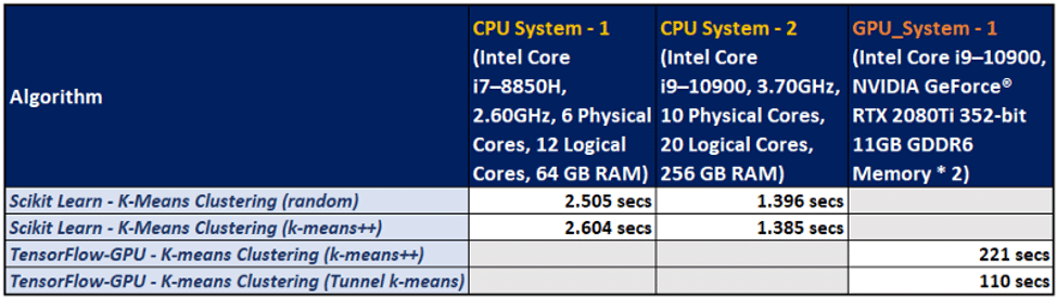
As we can observe in the comparison matrix, the GPU-powered system has a distinctive performance advantage by means of execution times.
The full implementation code and Jupyter Notebook is available on my GitHub.
Reading Time: 9 minutes
Don’t miss out the latestCommencis Thoughts and News.

17/03/2020
Reading Time: 9 minutes
A Benchmark: K-Means Algorithms for Scikit-Learn and TensorFlow-GPU
When you would like to have a deeper understanding of a phenomenon, one approach can be putting them in groups to make it easier to comprehend. As an example, you might want to view movies by title, while another person might view it by genre. How you decide to group them guides you to learn more about them.
In machine learning, dividing the data points into a certain number of groups is called clustering. These data points do not have initial labels. For that reason, clustering is the grouping of unlabeled data points into groups to figure them out in a more meaningful way.
There exist three kinds of clustering as Hierarchical Clustering (Divisive, Agglomerative), Partitional Clustering (Centroid, Model-Based, Graph-Theoretic, Spectral) and Bayesian Clustering (Decision Based, Nonparametric). In this post, we will be using Partitional Clustering>Centroid as the clustering algorithm.
For more deeper look for clustering techniques, please visit MIT-edu notes.
Throughout this post, the aim is to compare the clustering performances of Scikit-Learn (random, k-means++) and TensorFlow-GPU (k-means++, Tunnel k-means) algorithms by means of their execution times and print them in a comparison matrix by providing corresponding system specs. Since the content of the data is not the focus of this benchmark study, the required data sets will be randomly generated.
Don’t miss out the latestCommencis Thoughts and News.
K-means Clustering
The purpose of k-means clustering is to partition some number of observations n into k number of centroids in a non-overlapping manner. The number of data points are expected to be as homogeneous as possible inside the cluster and as heterogeneous as possible outside the cluster. For more theoretical explanations, please kindly visit this webpage.
The algorithm works when a group of center points is available by following the below steps:
- Existing clusters are updated in order to include the nearest data points in distance to every centroid.
- The center points are iteratively recomputed as the average of all data points involving in a cluster.
Throughout this post, three different environments (2 different CPU-powered system, 1 GPU-powered system) will be tested. The system specs are added below.
First CPU-Powered System Specs:
Processor: Intel(R) Core(TM) i7–8850H
Processor Speed: 2.60 GHz
Physical Cores: 6
Logical Processors: 12
Physical Memory (RAM): 64 GB
Second CPU-Powered System Specs:
Processor: Intel(R) Core(TM) i9–10900
Processor Speed: 3.70 GHz
Physical Cores: 10
Logical Processors: 20
Physical Memory (RAM): 256 GB (8 x 32GB DDR4 3000 MHz)
GPU-Powered System Specs:
Processor:Intel(R) Core(TM) i9–10900
Processor Speed: 3.70 GHz
Graphics Processors (GPU): NVIDIA GeForce® RTX 2080Ti 352-bit 11GB GDDR6 Memory (2)
1. CPU-based K-means Clustering
Central Processing Unit (CPU) is the crucial part computer where most of the processing and computing performs inside.
For the further coding part, we will be using the Python programming language (version 3.7). Both PyCharm and Jupyter Notebook can be used to run Python scripts. For the ease of use, Anaconda can be installed since it includes all required IDE’s and vital packages with itself.
As an initial step, we will be installing the required packages that will be required CPU implementation.
pip install psutil
pip install numpy
pip install matplotlib
pip install scikit-learn
After installing psutil, numpy, matplotlib, sklearn we will import the packages in order to be able to benefit from their features.
import platform
import time
import psutil as ps
import platform
from datetime import datetime
import numpy as np
import matplotlib.pyplot as plt
from sklearn.cluster import KMeans
Before start clustering, CPU information and their current CPU usage percentages can be checked with the following code snippet.
print("Physical cores:", ps.cpu_count(logical=False))
print("Logical cores:", ps.cpu_count(logical=True),"\n")

print("CPU Usage Percentages:", "\n")
for i, percentage in enumerate(ps.cpu_percent(percpu=True)):
    print(f"CPU {i}: {percentage}%")

print("\n")
print(f"Current CPU Usage in Total: {ps.cpu_percent()}%")
There are two types of k-means algorithm that is existent within Kmeans() function with the parameter “init= random” or “init=kmeans++”. In below, firstly “init = random” which stands for selecting k observations in a random manner will be tested.
“n_clusters” parameter stands for the number of clusters the algorithm will split into. When we assign “n_clusters” into “100”, it signals algorithm to distribute all data points into most appropriate 100 centroids. To be able to control the randomness in every run, “random_state” parameter shall be set to an integer number; otherwise, a different random group will be selected in every run which will be harder to compare with the previous outputs.
kmeansRnd = KMeans(n_clusters=100, init='random',random_state=12345)
After setting cluster parameters, random numbers are generated with 5 columns and 500 K rows.
CPU_Test_1 = np.random.normal(size=(500000,5))
Now, we have 5-columned and 500 K-rowed randomly generated data. With “fit_predict” function, cluster centers and cluster indexes will be calculated for each data point by feeding our data named “CPU_Test_1”.
kmeansRnd.fit_predict(CPU_Test_1)
Visualization of the samples and the number of clusters are added by using “plotly” package of python. The results of this plotting script are added at the end of the system-based results in the upcoming sections of the post while depicting the data points and the clusters.
plt.scatter(CPU_Test_1[:,0], CPU_Test_1[:,1], s=1)
plt.scatter(kmeans.cluster_centers_[:,0], kmeans.cluster_centers_[:,1], s=5, c="r")
plt.title("K-means (Random) with Scikit Learn", "\n")
plt.show()
Execution times of the algorithms can be tracked by adding the following code lines outside of our algorithm.
start_time = time.time()
# ... clustering code block
end_time = time.time()
print(end_time - start_time)
1.1. K-means (random) Clustering with Scikit-Learn
Scikit Learn K-means — random algorithm chooses the first center cluster in a random way which might cause a higher in-cluster variance compared to k-means++ algorithm.
First CPU-Powered System Results:
Algorithm Execution Time: 2505.26 seconds
Clusters Visualization: Blue Dots (Data Points), Red Dots (Clusters)
Second CPU-Powered System Results:
Algorithm Execution Time: 1395.10 seconds
Clusters Visualization: Blue Dots (Data Points), Red Dots (Clusters)
1.2. K-means (kmeans++) Clustering with Scikit-Learn
Scikit Learn K-means — kmeans++ algorithm chooses the first center cluster in a more logical way which can lead to a more accelerated clustering performance afterward.
First CPU-Powered System Results:
Algorithm Execution Time: 2603.74 seconds
Clusters Visualization: Blue Dots (Data Points), Red Dots (Clusters)
Second CPU-Powered System Results:
Algorithm Execution Time: 1384.73 seconds
Clusters Visualization: Blue Dots (Data Points), Red Dots (Clusters)
2. GPU-based Clustering
Tensorflow library is developed to be used for massive volumes of numerical computations. It supports both CPU and GPU according to the installed version of your environment. If you wish to enable your GPU(s), the version that is needed to be installed is TensorFlow-GPU.
pip install tensorflow-gpu
In order to be able to test the availability of GPU information by using TensorFlow library, the following code snippet can be used.
import tensorflow as tf
config = tf.compat.v1.ConfigProto()
tf.config.list_physical_devices('GPU')
Output:
After viewing GPU information by using the below script, more detailed device information, including CPU(s), can be printed.
from tensorflow.python.client import device_lib as dev_lib
print (dev_lib.list_local_devices())
Output:
2.1. KMeansTF (kmeans++) Clustering with TensorFlow-GPU
TensorFlow k-means algorithm routes the negative effects of randomly generated initial centroid by iteratively optimizing in-cluster variance.
GPU-enabled Tensorflow k-means algorithm can be used by installing the following kmeanstf package.
pip install kmeanstf
After installing the required package, the following algorithm will be running in a GPU-based environment. Results are added after system specs.
from kmeanstf import KMeansTF
start_time = time.time()
kmeanstf = KMeansTF(n_clusters=100, random_state=12345)
GPU_Test = np.random.normal(size=(500000,5))
kmeanstf.fit(GPU_Test)
end_time = time.time()
print('Kmeans++ execution time in seconds: {}'.format(end_time - start_time))
GPU-Powered System Specs:
Algorithm Execution Time: 219.18 seconds
Clusters Visualization: Blue Dots (Data Points), Red Dots (Clusters)
2.2. TunnelKMeansTF Clustering with TensorFlow-GPU
Tunnel k-means algorithm has the capability to achieve non-local shifts between clusters to find the most optimum centroids for each data point.
start_time = time.time()
kmeansTunnel = TunnelKMeansTF(n_clusters=100, random_state=12345)
GPU_Test = np.random.normal(size=(500000,5))
kmeansTunnel.fit(GPU_Test)
end_time = time.time()
print('Tunnel Kmeans execution time in seconds: {}'.format(end_time - start_time))
GPU-Powered System Specs:
Algorithm Execution Time: 107.38 seconds
Clusters Visualization: Blue Dots (Data Points), Red Dots (Clusters)
3. Final Comparison Matrix
To have a clearer understanding of the outputs of the algorithms, a matrix table is generated.
As we can observe in the comparison matrix, the GPU-powered system has a distinctive performance advantage by means of execution times.
The full implementation code and Jupyter Notebook is available on my GitHub.


